-
Články
Top novinky
Reklama- Vzdělávání
- Časopisy
Top články
Nové číslo
- Témata
Top novinky
Reklama- Videa
- Podcasty
Nové podcasty
Reklama- Kariéra
Doporučené pozice
Reklama- Praxe
Top novinky
ReklamaChild Mortality Estimation: Appropriate Time Periods for Child Mortality Estimates from Full Birth Histories
Background:
Child mortality estimates from complete birth histories from Demographic and Health Surveys (DHS) surveys and similar surveys are a chief source of data used to track Millennium Development Goal 4, which aims for a reduction of under-five mortality by two-thirds between 1990 and 2015. Based on the expected sample sizes when the DHS program commenced, the estimates are usually based on 5-y time periods. Recent surveys have had larger sample sizes than early surveys, and here we aimed to explore the benefits of using shorter time periods than 5 y for estimation. We also explore the benefit of changing the estimation procedure from being based on years before the survey, i.e., measured with reference to the date of the interview for each woman, to being based on calendar years.Methods and Findings:
Jackknife variance estimation was used to calculate standard errors for 207 DHS surveys in order to explore to what extent the large samples in recent surveys can be used to produce estimates based on 1-, 2-, 3-, 4-, and 5-y periods. We also recalculated the estimates for the surveys into calendar-year-based estimates. We demonstrate that estimation for 1-y periods is indeed possible for many recent surveys.Conclusions:
The reduction in bias achieved using 1-y periods and calendar-year-based estimation is worthwhile in some cases. In particular, it allows tracking of the effects of particular events such as droughts, epidemics, or conflict on child mortality in a way not possible with previous estimation procedures. Recommendations to use estimation for short time periods when possible and to use calendar-year-based estimation were adopted in the United Nations 2011 estimates of child mortality.
Published in the journal: . PLoS Med 9(8): e32767. doi:10.1371/journal.pmed.1001289
Category: Research Article
doi: https://doi.org/10.1371/journal.pmed.1001289Summary
Background:
Child mortality estimates from complete birth histories from Demographic and Health Surveys (DHS) surveys and similar surveys are a chief source of data used to track Millennium Development Goal 4, which aims for a reduction of under-five mortality by two-thirds between 1990 and 2015. Based on the expected sample sizes when the DHS program commenced, the estimates are usually based on 5-y time periods. Recent surveys have had larger sample sizes than early surveys, and here we aimed to explore the benefits of using shorter time periods than 5 y for estimation. We also explore the benefit of changing the estimation procedure from being based on years before the survey, i.e., measured with reference to the date of the interview for each woman, to being based on calendar years.Methods and Findings:
Jackknife variance estimation was used to calculate standard errors for 207 DHS surveys in order to explore to what extent the large samples in recent surveys can be used to produce estimates based on 1-, 2-, 3-, 4-, and 5-y periods. We also recalculated the estimates for the surveys into calendar-year-based estimates. We demonstrate that estimation for 1-y periods is indeed possible for many recent surveys.Conclusions:
The reduction in bias achieved using 1-y periods and calendar-year-based estimation is worthwhile in some cases. In particular, it allows tracking of the effects of particular events such as droughts, epidemics, or conflict on child mortality in a way not possible with previous estimation procedures. Recommendations to use estimation for short time periods when possible and to use calendar-year-based estimation were adopted in the United Nations 2011 estimates of child mortality.Introduction
Tracking Millennium Development Goal 4, which sets a target of reducing child mortality by two-thirds between 1990 and 2015, requires that the under-five mortality rate (also denoted in the literature as U5MR or 5q0), be estimated precisely and accurately. Moreover, child mortality is an important indicator of the performance of the public health system of a country. Demographic and Health Surveys (DHS) surveys and similar surveys that collect full birth histories are one of the chief sources of estimates of under-five mortality, deriving such estimates from women's own reports of their complete birth histories.
The DHS surveys were originally designed for samples of 5,000–6,000 eligible women [1]. Measures of child mortality have traditionally been reported for 5-y time periods, since time periods shorter than 5 y often result in sampling errors that are too large because estimates are based on the deaths that occur during the particular time spans. Many recent surveys have had sample sizes much larger than required by the original design, and these larger sample sizes may make it possible to use time periods shorter than 5 y for child mortality estimates.
Estimates for short time periods have the benefit that trends and deviations from trends may be ascertained with some detail. The mortality effects of particular events, such as a drought, hurricane, or the outbreak of war, may be tracked if the time period is sufficiently short. Moreover, recent major changes in the pace of change of child mortality may be discovered earlier than if long time periods are used for estimation.
The tracking of the Millennium Development Goals is partly global, but the responsibility for meeting the goals lies with each country. Moreover, regardless of international goal setting, countries need to monitor the development of their child mortality level as an important indicator of the performance of their public health system. Global tracking of child mortality can be considered to be served by the current 5-y period of estimation, since short-term and local effects might obscure the overall trend. However, the overall trends for the different countries are constructed by smoothing the data from several surveys [2], so the trend estimates can be relatively smooth even if the estimates from particular surveys reflect specific events or random fluctuations observed in a country. Thus, using short estimation periods in the estimation from individual surveys can serve both the overall trend analysis and the short-term concerns that are of interest for individual countries.
The term “time period” in the context of child mortality estimation actually has two meanings. The first is the duration of the period for which an estimate is derived, 1 y, 2 y, and so on. The second is somewhat subtle. The usual practice in DHS surveys is to estimate mortality based on the concept of “years before the survey.” That is, the estimation period is measured with reference to the time of the interview of each individual woman. As a consequence, the survey estimates for a period will actually cover a longer period than the apparent number of years in the period since the fieldwork may last from 2 mo to nearly a year. An alternative is to measure time in calendar years independent of when each woman was interviewed. The benefit of the traditional DHS approach is that it allows estimates into the fieldwork period of the survey, while the benefit of the calendar year approach is that it is provides a much clearer time reference. Thus, this paper will explore the consequences of using calendar-year-based estimates rather than estimates based on the time of the interview of each woman.
We proceed by considering criteria for when the sampling variability of an estimate is sufficiently small for tracking the levels and trends in child mortality, as well as the theory behind how to select appropriate time periods when sampling phenomena that fluctuated in time. We then give an overview of how DHS surveys are designed and how child mortality estimates and their sampling errors are computed. We then compute child mortality measures and their sampling errors for available DHS surveys in order to ascertain the conditions that allow the use of short time periods.
One way to determine appropriate time periods is to consider the standard errors of the estimates, and then reject any estimate if its standard error is too high. Since the standard error is scaled to what is measured, a common approach used in survey statistics and in other fields is to consider the coefficient of variation, i.e., the standard error divided by the estimate, expressed as a percentage or as the unmodified ratio [3],[4]. Strictly speaking, the coefficient of variation may be thought of as a population parameter, and as “relative standard error” or “coefficient of variation estimate” when calculated from samples [5]. Common usage is nevertheless to use the term “coefficient of variation” also for sample estimates.
It is commonly assumed that an estimate can be accepted for use or publication if its coefficient of variation is less than a given value, usually less than 5% or 10% of the estimate. Nevertheless, the rule of thumb of 5% or 10% is somewhat arbitrary, as is the case with many statistical rules of thumb, such as the 95% confidence interval [6]. Kish [7] agrees with Hansen et al. [8] that coefficients of variation larger than 0.2 (i.e., 20%) indicate a danger of unstable estimates, and notes that in his own practice “whenever the program found cv(x)>0.1 it printed out in red letters STOP, LOOK, AND DO SOMETHING” (“cv” is coefficient of variation) [7]. Hansen et al. [8] adopt 10% as a “working rule.” In a somewhat more bureaucratic tone, the Eurostat sampling guidelines require the national statistics offices of member states to ensure that the coefficient of variation is lower than 8% in reported estimates from national surveys [9].
Despite the fact that what exact level one should choose as a cutoff may be uncertain, the reason for not accepting high coefficients of variation is clear cut. Like the estimate of child mortality itself, the standard error as observed in a survey is a sample statistic. A large standard error (and correspondingly large coefficient of variation), means that one does not really know where within the confidence interval the true value lies, but only that the confidence interval is wide, because the statistics used to compute it are uncertain. When samples are small, both the estimates and their variance estimates become unstable. This was to a large extent Kish's concern in the quotation above. But when the coefficient of variation is smaller than the level implying instability, there is no obvious statistical reason for choosing between the conventional 5% or 10% or the Eurostat's 8%.
In addition to the purely statistical issue, there is a substantive issue of importance in choosing an acceptable level for the coefficient of variation. For a child mortality rate of 100 deaths per 1,000, a 10% coefficient of variation would give a 95% confidence interval of roughly 80–120, while a 20% coefficient of variation would give a 95% confidence interval of 60–140. The latter is way too large if one wants to estimate change from one period of estimation to the next, or indeed for estimating the level itself. But, ultimately, the question is one that revolves around what is needed for specific purposes.
The appropriate time period for analysis is not simply the smallest that the sample size can support. If one assumes the absence of bias in a given child mortality measure estimate, in principle the appropriate time period is determined by the level of child mortality, the level of fertility, the sample size (and the sample design), and the variation in child mortality over time. The Shannon-Nyquist sampling theorem [10] describes the relationship between the frequency of a signal and how often the signal needs to be measured in order to be accurately represented. The more frequent the variation, the shorter the period needed in order to accurately portray it. In general, if there is no fluctuation with a frequency higher than B, then one should sample at intervals that are shorter than 1/(2B). For example, to accurately describe mortality fluctuations that occur every second year, i.e., with a frequency equal to 0.5, one would need to sample with an interval no longer than a year (1/(2×0.5) = 1). The frequent sampling required by the sampling theorem is clearly unrealistic given the sampling error in the case of child mortality estimates.
The Shannon-Nyquist sampling theorem assumes measurements at instants. In the case of child mortality measurements, that is not possible, as child mortality estimates are, again for sample size reasons, not measured at instants, but for periods that are long compared to possible fluctuations in mortality level. If child mortality varies regularly with 5 y between peaks, then a series of 1-y periods of estimation is able to reconstruct the curve form relatively well, as shown by the step curve in Figure 1.
Fig. 1. Effects of choice of period on estimates. 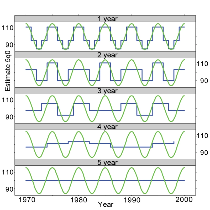
The figure shows a cosine curve (green lines) with a 5-y periodicity and average estimates based on 1- to 5-y periods (blue lines). Even with a 1-y estimation period there is some distortion in terms of peaks and troughs, if one considers that child mortality is a continuous smooth function of time. With a 2-y period more major distortions appear, because the periodicity of the measurements does not match the periodicity of the variation. This is even more pronounced with 3 - and 4-y periods, and with 5-y periods the original variation is not visible at all. The scenario shown in Figure 1, with a regular fluctuation of mortality, may be that which will be most distorted, since the regularity forces long periods to average out fluctuation. With a 5-y period, a peak during a single year or two followed by a return to a baseline will be detectable, although the importance of the peak will be understated.
The Rwanda 2000 DHS survey provides an empirical example of the issues at hand. The birth history recorded in the survey covers the 1994 genocide. Although the massacres took place mainly from April to July, effects on child mortality may have lasted longer. As can be seen in Figure 2, while the 1994 events are somewhat detectable on the 5-y period plot, the effect is clearly visible on the 1-y period plot, showing that the 5-y estimates seriously understate the mortality increase, even when one disregards selection effect issues such as that children whose mothers were killed, and who therefore were not interviewed in 2000, must have had a much higher risk of death than other children. The 2-y trend line also shows a substantial flattening of the trend compared to the 1-y trend, illustrating empirically the theoretical plot in Figure 1.
Fig. 2. 5q0 and confidence intervals for the Rwanda 2000 DHS survey. 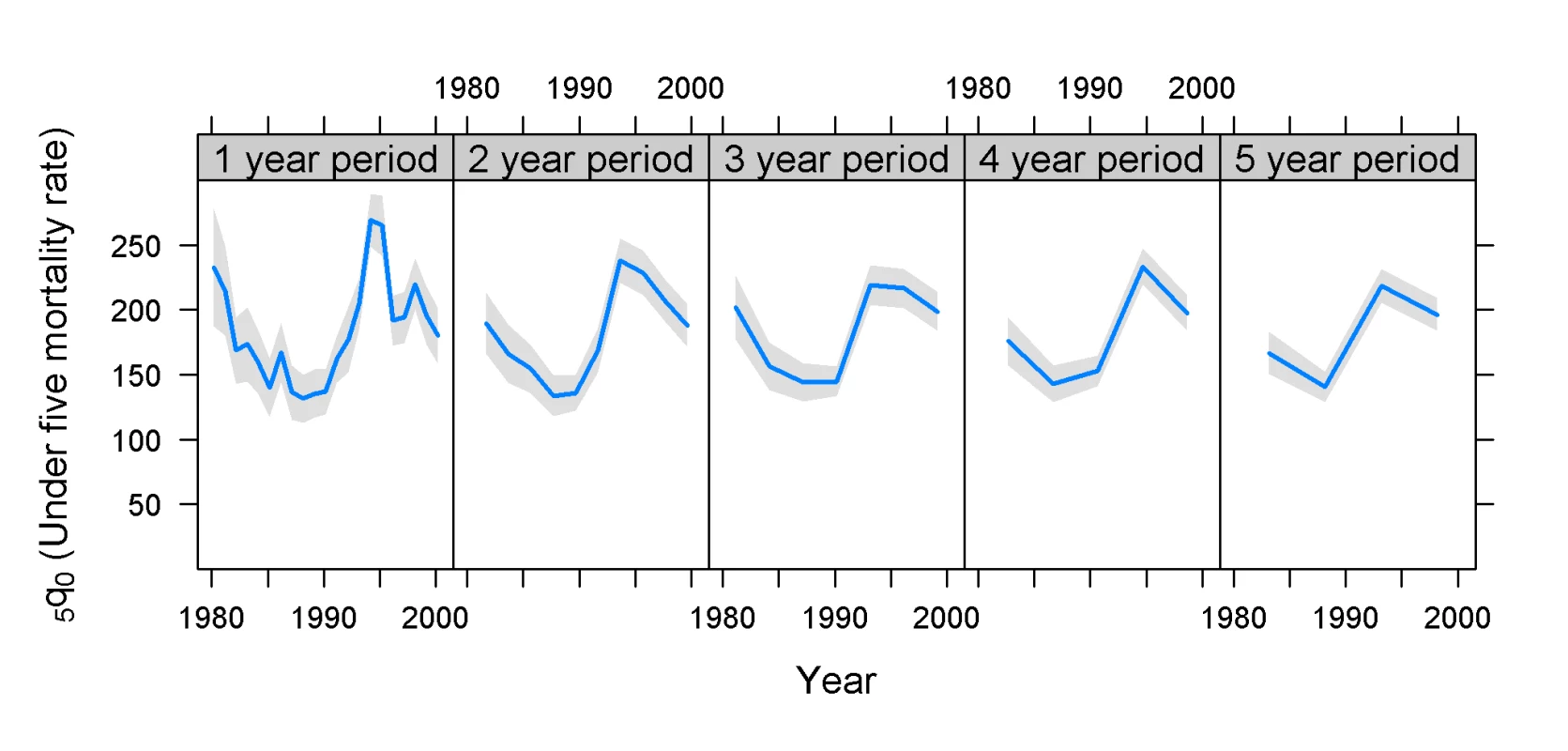
Estimates based on years before the survey. The distortion of the estimates is a problem that pertains not only to the shape of the trend lines of the mortality measures, but also—as the literature within economics indicates—to the issue that the coefficients of models based on the long time periods may be biased [11], in a way that is similar to misspecification error or ecological fallacy. This is a problem for models that use aggregated child mortality measures, such as attempts to create models of the relationship between gross domestic product per capita and child mortality for countries (e.g., [12],[13]) or models that aim to describe the relationship between conflict and child mortality levels (e.g., [14],[15]), but not for models focusing on finding covariates for individual child deaths.
A few observations follow from this exposition. First, sample sizes and mortality levels constrain how short a period can be used for estimation of child mortality measures. Second, having a large sample and using it to estimate child mortality measures with long observation periods is not optimal, because if mortality fluctuates, then significant bias may be a result. Thus, it may be better to trade lower precision (higher variance) in the estimate for higher accuracy (reduced bias) than to assume that a 5-y estimation period is always preferable. The problem remains, however, how that trade-off should be calibrated, and that will be addressed in the rest of this article. The purpose of this article is to determine appropriate time periods for child mortality estimates from full birth histories, given various sample sizes. Thus, it tries to answer the question of whether, given the increased sample sizes in recent years, we are wasting information by sticking to the estimation procedures that were developed for smaller samples.
Methods
Data Sources
The data used in this analysis were datasets that were publicly available from DHS, i.e., they could be downloaded from the Measure DHS website (http://www.measuredhs.com/data/available-datasets.cfm) without special permission from the country in question. Surveys that were carried out after 1 January 1985 and had data released before 31 October 2010 were included (surveys before 1990 do not appear to include sampling stratum information; a complete list of the surveys used is in Table S1). The data were not edited or altered in any way, except in the case where a dataset had one or more sampling strata consisting of only one cluster. In such cases each stratum in question was merged with an adjacent stratum or with a nearby stratum that also had only one cluster, i.e., employing the so-called collapsed stratum technique [16]. This will tend to overstate variance slightly. In some cases we did not feel confident that we had understood the stratification of the survey properly (e.g., Egypt 2005), and such surveys were dropped from the analysis. In total, 207 surveys were retained for analysis.
Rather than using exact dates in the estimation, DHS uses so-called century month coding, in which dates are converted into the number of months since January 1900. Some surveys, such as the Nepali and Ethiopian ones, use national calendars. These were recalculated according to the standard DHS coding and the Gregorian calendar. DHS data files do not contain the day part of dates, and therefore the conversion can be only approximate.
DHS Survey Design
The DHS surveys generally employ a two-stage stratified sampling design [1]. The sample is usually explicitly stratified by major administrative regions of the country in question, and also by urban and rural location. The allocation of the sample varies, and may be disproportionate in order to ensure adequate reporting domains, although proportionate allocation is preferred. The samples are very often implicitly stratified by geographic location within the explicit strata. Primary sampling units (PSUs) are most often census enumeration areas, consisting of 50 to 300 households. They are selected with probability proportionate to their size, as measured by their number of households, usually derived from the latest census of the country in question. If the PSUs are large then they are usually segmented, and only one segment is selected with probability proportionate to its number of households. PSUs (or segments) are always mapped, and a current list of households is created before the selection of households takes place by linear systematic sampling. Depending on the survey, and sometimes on geographic location within a specific survey, about ten to 20 households are selected in each PSU. As noted above, DHS surveys were designed for a sample size of 5,000–6,000 eligible women or approximately the same number of households, but many surveys have had larger samples, with those of India and Pakistan being the largest, with more than 100,000 households. Since 2005, the median sample size has been over 10,000 households, corresponding to an increase of roughly 3,000 households since 1990–1994 (Table 1).
Tab. 1. Sample Sizes for DHS surveys, 1985–2010. 
Based on output from the Measure DHS STATcompiler, and relevant survey reports when data were unavailable from the compiler. Sampling weights are calculated so that they account for the details of the design. Although the DHS design is in principle self-weighting within the explicit strata, weight variations do occur because the estimate of the PSU sizes from the sampling frame may differ from the actual number found in the PSUs during the mapping and listing. Moreover, weight variation naturally occurs between strata that have different overall sampling rates.
Mortality Estimation from Full Birth Histories
Full birth histories are taken from all women aged 15–49 y in most surveys, although some, principally in the Middle East and southern Asia, define only married women in the 15 - to 49-y-old group as eligible. Both usual residents of the households and visitors are used in the estimation.
The DHS estimates of child mortality are calculated using a synthetic cohort approach [17]. The age span from 0 to 5 y is split into eight groups, 0 to 30 d and 1 to 2, 3 to 5, 6 to 11, 12 to 23, 24 to 35, 36 to 47, and 48 to 59 mo. Survival probabilities from the beginning to the end of each age group are calculated, and then the appropriate measures are calculated as the product of the composite age rates.
DHS Variance Estimates
Estimates of variance for child mortality estimates from full birth histories collected through a typical household survey are somewhat involved. That is both because the various mortality ratios are computed in a complex fashion as described above, so that working out their variance estimator would be practically impossible, and because the sampling design is complex, i.e., includes unequal weights, clustering, and stratification, resulting in estimators that are not linear.
The variance estimates in the DHS reports have been calculated with a jackknife procedure. The basic premise of this method is that the realized sample can be seen as a good approximation of the population distribution, and that repeated samples from the sample can be made. The distribution of the estimates made from these subsamples will then reflect the sampling variability. While several methods based on this premise exist, the unique characteristic of the jackknife approach is that subsamples are formed by deleting one sampling unit from the sample, calculating the estimate, replacing the deleted unit, and then repeating the procedure with the next sampling unit. Thus, a number of replicate estimates equal to the number of sampling units is formed, and the variance is basically the variance of the distribution of replicates.
In jackknife cluster samples, the ultimate clusters, rather than the last stage sampling units, are used. Thus, for example, with a sample of 368 clusters and 24,000 births, 368 replicates are computed, not 24,000.
According to the DHS sampling manual [1] and the various country reports, the formula used for the variance estimate is
where k is the number of ultimate clusters, r is the estimate from the full sample, and r(i) is the estimate from the reduced sample of k−1 clusters, when cluster i is excluded.A characteristic of the variance estimator as employed by DHS is that it disregards stratification. Therefore, it likely overestimates variance, at least in samples where strata allocations are more or less proportional to the stratum sizes. A test on the 2002 DHS survey for Eritrea confirms that it was indeed the unstratified estimator that was used.
An alternative variance estimator is the JKn variance estimator used by Westat's WesVar software [18] and by SUDAAN [19], and described by Wolter [16]. The stratified JKn procedure for estimating variance is very similar to that of the unstratified version, i.e., it deletes and replaces each ultimate cluster in turn. However, when a cluster is omitted, the weights of the other clusters in the stratum are adjusted by a factor of nh/(nh−1), where nh is the number of clusters in the stratum. Then, the actual variance estimate is calculated as given below, where hk is (nh−1)/nh:
Note that in this case ri is the actual estimate from the i-th replicate, i.e., without the transformation applied in the formula used by DHS. The DHS formula and Equation 2 are in fact equivalent: if the adjustment to the weights and the hk factor are not applied, the two formulas yield the same result. Thus, the difference is the adjustment for stratification. The formula that DHS uses is the original version as described by Quenouille, the inventor of the method [16]. Neither the DHS version of the variance estimate nor the stratified version includes a finite population correction. In general, sampling rates in DHS surveys are too small for this to matter.The differences in standard errors between the estimates that DHS presents and those taking stratification into account are on the order of 10% or less, since the variances of the child mortality measures usually do not differ all that much between strata.
The mortality estimates and standard errors were produced by a program written in Delphi (Embarcadero RAD Studio XE). For each data source, estimates for 1-, 2-, 3-, 4-, and 5-y periods were calculated as far back in time as was possible for each survey, given the length of the birth histories. The estimates of childhood mortality for 5-y periods before the survey match exactly those produced by the Measure DHS online statistics compiler (STATcompiler) or the DHS final reports for datasets that are not represented in the compiler output. Delphi was chosen because the system produces compiled code. It is therefore much faster than the interpreted code used by R, Stata, or SPSS. The program reads comma-separated or Excel files exported from the original DHS data files. It is available from the authors on request. Computed estimates from the DHS surveys used in our analysis are found in Tables S2 and S3.
Results
Regardless of the length of the estimation period, 75% of the estimates of 5q0 have a coefficient of variation below 14%, and half below 10%. For estimation for periods of 3 y and more, the estimate of the coefficient of variation is less than 10% in 75% of the cases (Figure 3; Table 2). Nevertheless, the distribution within each period is highly skewed, with a few very high coefficients. In general, the outliers are surveys that have small sample sizes, represent estimation periods long before the survey date, have low fertility, or have low mortality, but there are some exceptions to this pattern.
Fig. 3. Distribution of coefficient of variation of 5q0 by length of period of estimation. 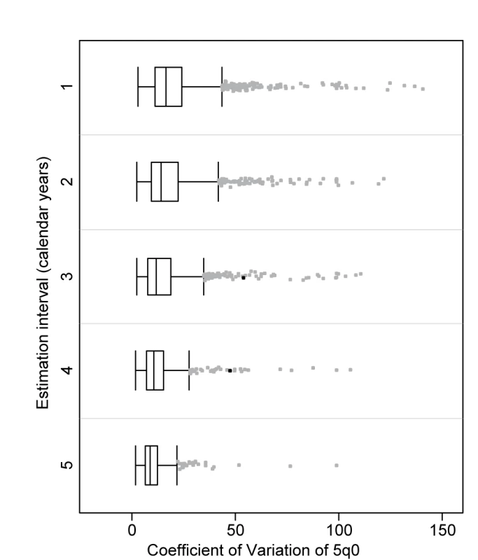
Only estimates for periods 20 y or less before the survey were included. Two extreme outliers have been excluded from the graph. Tab. 2. Distribution of coefficient of variation for 5q0 by length of period. 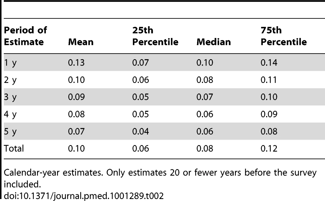
Calendar-year estimates. Only estimates 20 or fewer years before the survey included. The results are highly determined by sample size, mortality level, and fertility (Figures 4 and 5; Table S1). To some extent, fertility can be used as a proxy for mortality level, since countries with high fertility usually also have high child mortality. In general, with the total fertility rate at 5.5 births per woman or higher, all realistic sample sizes, including small ones, make the estimation of 5q0 for single-year periods at least 10 y back from the survey date feasible if a coefficient of variation of less than 10% is the criterion. At medium fertility levels, 3.5–5.5 births per woman, one would need a sample of at least 8,000 to be able to estimate 5 y back with 1-y periods, while 12,000 would be required for estimating 10 y back. At fertility levels lower than 3.5 births per woman, estimation of 5q0 with samples of less than 8,000 households appears to be ill-advised, regardless of the period for estimation. At low fertility levels and with small samples, the only estimate that can be made with confidence in most cases is 5q0 for 0–4 y before the survey, and sometimes not even that (e.g., Kazakhstan).
Fig. 4. Mean number of contiguous years before survey allowing estimates with coefficient of variation less than 10%, by sample size, estimation period, and total fertility rate (births per woman). 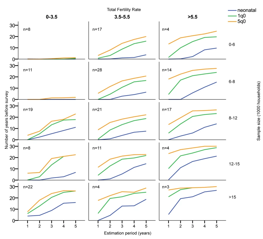
Estimates based on years before the survey. The number of surveys used for the estimates in each panel is indicated in the upper left corner of each. Fig. 5. Mean number of contiguous years before survey allowing estimates with coefficient of variation less than 5%, by sample size, estimation period, and total fertility rate (births per woman). 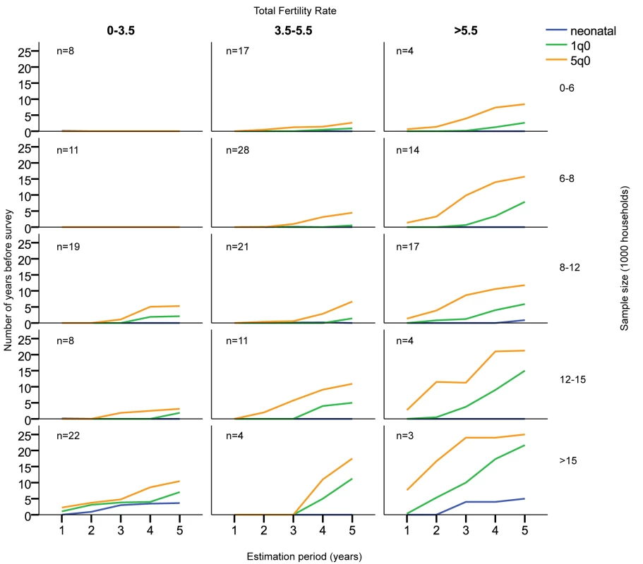
Estimates based on years before the survey. Estimates based on calendar years. The number of surveys used for the estimates in each panel is indicated in the upper left corner of each. One should note, however, that there are exceptions to the general rules of sample size and fertility. Sierra Leone 2008 has, for example, no estimate with a coefficient of variation lower than 10%. It is unclear why this is so, since Sierra Leone 2008 has a standard DHS sample design, with a sample size of 7,572 households and a total fertility rate of 5.1 births per woman.
Similar considerations pertain to neonatal mortality (formally, the number of deaths during the first 28 d after birth per 1,000 births, but estimated in DHS surveys and here as the number of deaths during the first month) and infant mortality (the number of deaths during the first year after birth per 1,000 births) estimates. Since the number of deaths observed in a period is smaller for these estimates, the number of years with low coefficients of variation is also fewer than for the 5q0 estimates. Nevertheless, if a coefficient of variation of less than 10% is the standard, then it is possible to produce mortality estimates 5 to 10 y back, even for neonatal mortality in high-fertility populations for most samples, but estimation further back than the most recent 5 y is likely to be unstable.
Not surprisingly in the case of neonatal mortality, the number of continuous years before the survey that can provide estimates with acceptable coefficients of variation is quite small regardless of the period used. For 1-y estimation periods, one needs samples of more than 15,000 households to be able to estimate back much in time.
If a coefficient of variation of less than 5% is the standard, then samples of more than 15,000 households are needed in order to make estimates for 1-y periods for 5q0, and neonatal and infant mortality can seldom be estimated at all (Figure 5; Table S1).
The results described above can also be seen graphically for each individual country survey. The general trend, regardless of sample size, is that the confidence intervals around the curves are quite narrow close to the survey date, and they then become wider the further away from the survey date the estimate is located. Mali 2001 (Figure 6) is an example of a survey of a high-mortality and high-fertility situation (5q0 of 200/1,000 or more; total fertility 5 y before the survey was 6.8 births per woman), with a relatively large sample (13,429 completed household interviews). Such a survey allows estimation for 1-y periods more than 20 y back in time using the 10% criterion. It is also a case where the period of estimation makes little difference, because the development of mortality has been relatively smooth.
Fig. 6. Estimates of 5q0 and confidence intervals for Mali 2001 DHS survey. 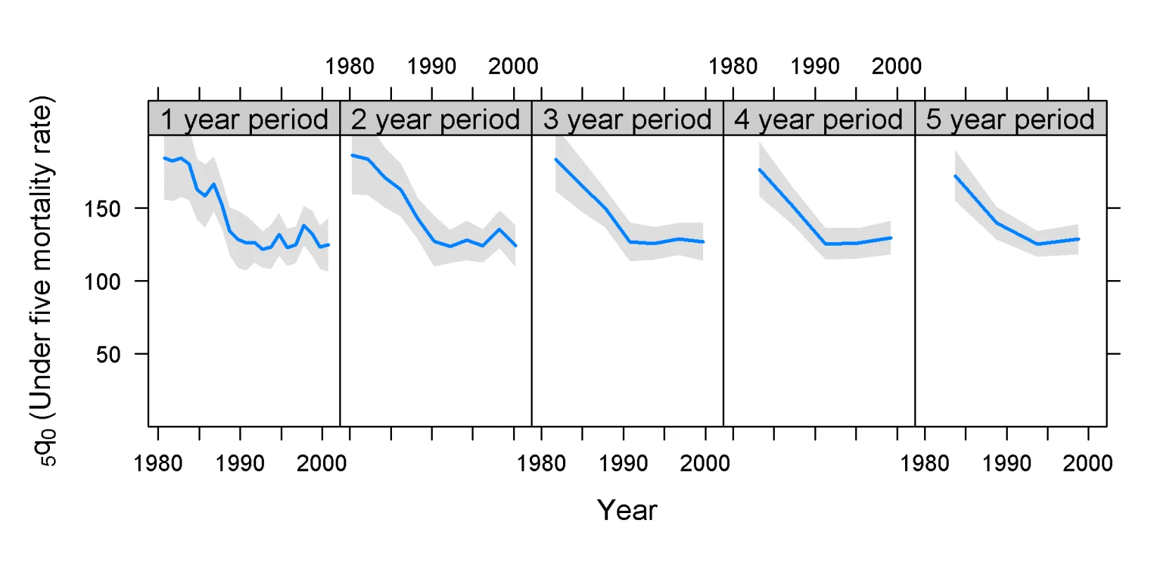
Sample size 12,439 households; total fertility rate 6.8 (births per woman). Estimates based on years before the survey. In contrast to Mali 2001, the Kazakhstan 1999 survey had a small sample, and the country had relatively low mortality and quite low fertility (Figure 7). The survey estimates have generally wide confidence intervals. The 1 - and 2-y estimates suggest a peak in child mortality around 1997 and then a decline, while the 5-y line suggests a slight recent increase.
Fig. 7. Estimates of 5q0 and confidence intervals for Kazakhstan 1999 DHS survey. 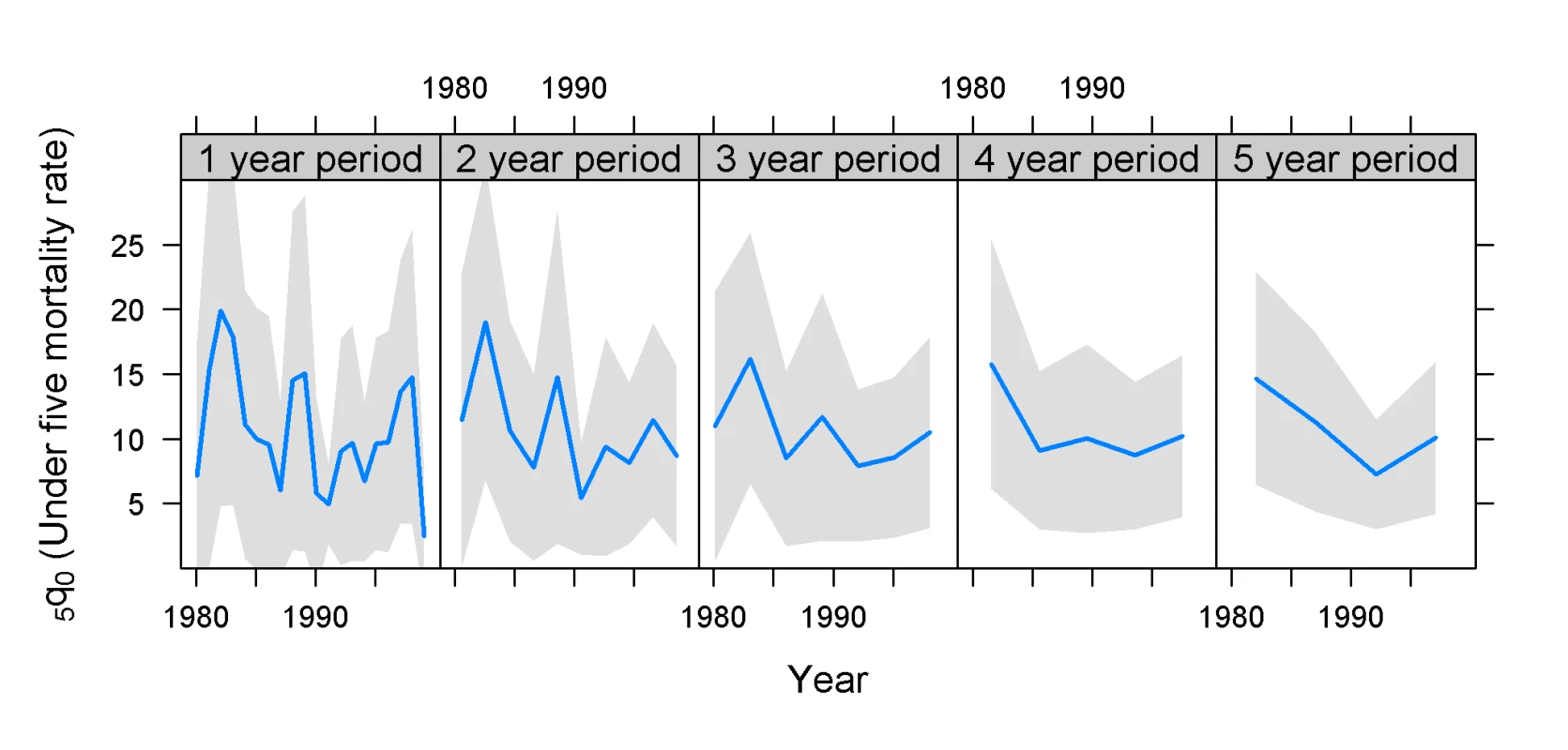
Sample size 5,841households; total fertility rate 2.0 (births per woman). Estimates based on years before the survey. Moldova 2005 (Figure 8) has twice the sample size of Kazakhstan 1999, and this is reflected in the more narrow confidence bands. Still, it is difficult to achieve really small coefficients of variation for surveys in countries with relatively low mortality and very low fertility.
Fig. 8. Estimates of 5q0 and confidence intervals for Moldova 2005 DHS survey. 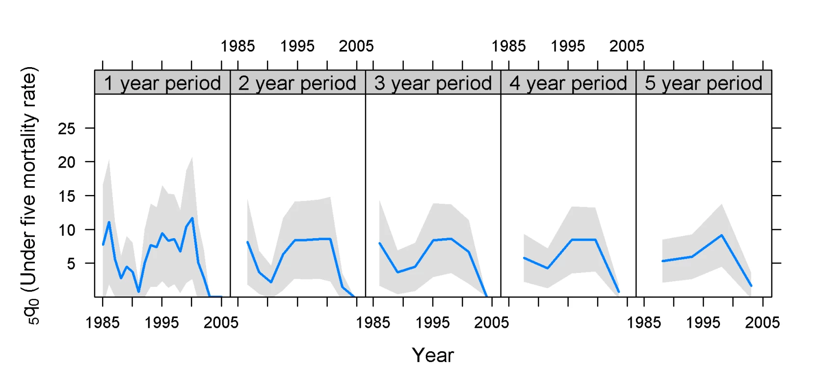
Sample size 11,095 households; total fertility rate 1.7 (births per woman). Estimates based on calendar years. The Zimbabwe 1999 data show a characteristic trumpet shape of the confidence bands, which is seen in many surveys: the further the estimate is from the survey date, the wider the estimate of the confidence band (Figure 9). The reason for this is that for estimates back in time, only a portion of the women interviewed provide data. Thus, children reported for 20 y ago were born to women who at the time were under 30 y. This reduces the sample size, and also introduces selection biases, since such estimates reflect the mortality of children born only to young mothers, and because it excludes children of women who have died.
Fig. 9. Estimates of 5q0 and confidence intervals for Zimbabwe 1999 DHS survey. 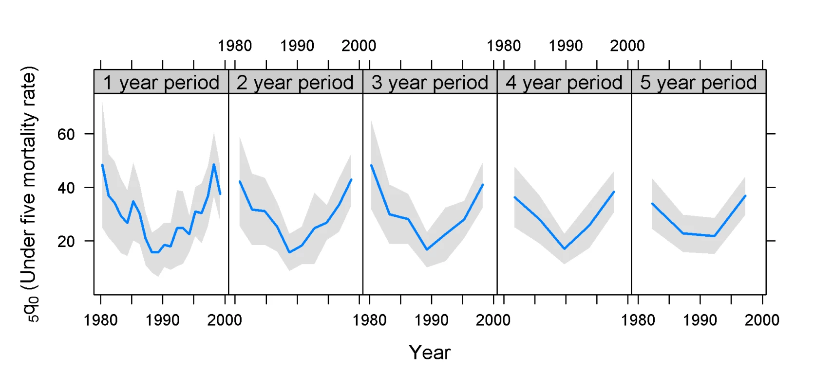
Sample size 6,372 households; total fertility rate 4.0 (births per woman). Estimates based on calendar years. Issues of Bias
As noted in the Introduction, focusing on the coefficient of variation overlooks the combined effects of bias due to long periods and sampling error. In principle, one can consider the mean square error, rather than the sampling error in isolation. If the bias and sampling error are uncorrelated, then the mean square error (MSE) is given by:
The square root of the mean square error, usually termed root mean square error, is then comparable to a standard error, but includes the effect of the bias. Thus, the root mean square error is a measure of the total uncertainty associated with the estimate.The problem is to estimate the bias. A simple approach is to assume that the difference between two estimates, e.g., for a 5-y period and a 1-y period, constitutes the bias of the longer period. That is certainly inaccurate, not the least because both estimates are subject to sampling error, and the 1-y estimate also may have some long-period bias. Moreover, the 1-y estimate is also biased because of selection effects, as noted before. With these caveats, one may reconsider the calculation of the root mean square error for the 5q0 mortality trend during the genocide period in Rwanda, as recorded by the 2000 DHS survey.
The root mean square error for the 5-y estimate (using the difference between the 1-y estimate for February 1994 and the 5-y period centered on February 1993 as a proxy for bias) is 51.2, while that for the February 1994 1-y period estimate remains 10.4, as the bias is assumed to be 0 (Table 3).
Tab. 3. Single-year and 5-y estimates of 5q0 and standard errors for the Rwanda 2000 DHS survey. 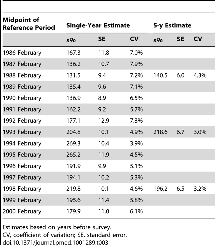
Estimates based on years before survey. The large root mean square error of the 5-y estimate appears credible when considered together with a graphical view of the development of 5q0 in Rwanda (Figure 10), with the data from the 2000 and 2005 DHS surveys (the 2007–2008 DHS survey shows a very different trend, and is disregarded here, while the 1992 DHS survey is consistent with the 2000 and 2005 surveys but irrelevant for the genocide period). A first observation that can be made from Figure 10 is that the 1-y period estimates from both the 2000 and 2005 surveys show clear peaks in 1994, although the 2005 survey shows one peak between the two peaks of the 2000 survey—most likely because of the difference in exactly when the time period of the estimate is centered. A second observation from the graph is that to some extent 1-y periods may remove some of the inconsistencies associated with trends based on the 5-y period estimates. The 5-y periods from both surveys show a leveling off of increasing mortality around the time of the genocide. The 2000 DHS survey suggests that this happened before the genocide, while the 2005 survey suggests that it happened after.
Fig. 10. Trends in <sub>5</sub><i>q</i><sub>0</sub> in Rwanda 2000 and 2005 DHS surveys using estimation periods based on years before the survey. 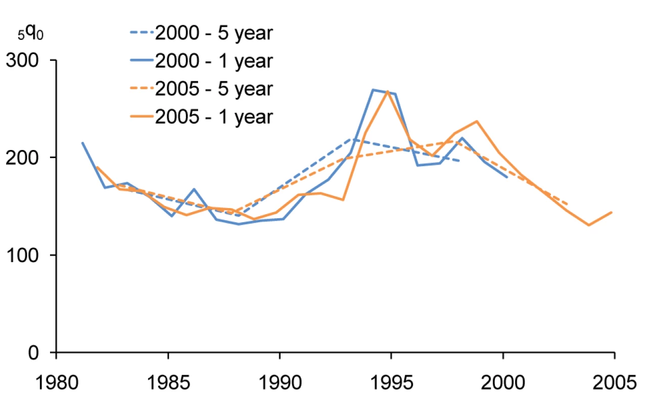
The preceding analysis implicitly makes three points. First, even though the 5-y period estimates in general have lower standard errors than the 1-y period estimates, the 1-y period estimates may be preferable, because of the potential bias that may occur in using the 5-y estimates. Second, one possible decision criterion is that when the mean square error (as calculated above) is larger for the 5-y estimate than for the 1-y estimate, the 1-y estimate is preferable. Third, if the coefficient of variation of the 1-y estimate is sufficiently low (i.e., at least lower than 10%), then the 1-y estimate should be preferred. In cases where the differences between the 5-y period estimates and the 1-y estimates are slight, the choice is largely irrelevant.
A further consideration is the time location of the estimates. As noted, the DHS estimates cover a longer calendar period than the estimation period, because the time reference is with respect to each individual interview date. This is a relatively minor consideration for 5-y periods, especially if the fieldwork period is short, but becomes an important consideration for the short estimation periods, such as 1 - and 2-y periods, especially in the context of rapidly changing mortality. The consideration is also becoming increasingly important as samples increase in size, since large surveys require longer fieldwork periods.
The effect of the time location can easily be seen by recomputing the estimates for calendar years rather than years before the survey. The midyear estimates of 5q0 computed from the Rwanda 2000 and 2005 surveys were, respectively, 208 and 192 for 1993, 281 and 260 for 1994, and 248 and 235 for 1995, i.e., a match that puts the yearly estimates squarely within each other's confidence intervals, and with peaks in the same years (Figure 11).
Fig. 11. Trends in <sub>5</sub><i>q</i><sub>0</sub> in Rwanda 2000 and 2005 DHS surveys using calendar-year estimation periods. 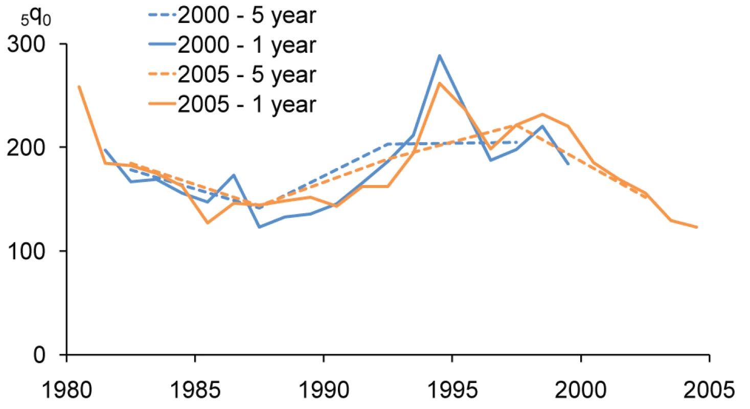
Since the Rwanda massacres took place within a calendar year, it is likely that estimates based on calendar year are more accurate than estimation based on years before the survey. But what works best for sudden changes in mortality is dependent on the actual time location of the sudden change. Nevertheless, fixing the estimates to calendar years rather than to years before the survey, which is anchored in the individual interview dates of the women providing the birth histories, has the benefit of making the estimates more directly comparable across surveys. The apparent inconsistencies between the 1-y estimates from the two Rwanda surveys, as well as between the 5-y period estimates, disappear with calendar-year-based estimation.
Discussion
Our analysis shows that whereas childhood mortality estimates based on 5-y periods of data have previously been the norm, the sample sizes presently employed in DHS surveys make it feasible to base the estimates on shorter periods. It also shows that using calendar years rather than years before the survey as a basis for estimation is useful because it brings out variation in child mortality in a clearer and more realistic manner.
Apart from the benefit in relation to tracking the Millennium Development Goals and the general benefit of avoidance of bias, there are three main benefits of this approach in relation to monitoring of public health. The first is that changes in mortality rates may be detected earlier. The second is that the relationship between child mortality rates and other events may be elucidated. One example is that of Rwanda, where the use of 5-y rates based on years before the survey seriously distorts the effect of the genocide on child mortality. Another example is the relationship between child mortality and outbreaks of some epidemic diseases, such as measles, which may be detected with the use of 1-y rates, but which will be undetectable with the use of 5-y rates. Finally, using short time periods for estimates, survey data may be used to establish consistency with other sources of child mortality estimates. Vital registration is often incomplete in developing countries, but one often assumes that the trends in vital registration data can be used for tracking fluctuation in child mortality [20]. This assumption is difficult to check with 5-y estimates from survey data, since vital registration typically provides data for single years, but the check can be carried out with single-year estimates.
For surveys with sample sizes larger than 8,000 households, it is possible in most cases to estimate child mortality for single years about 10 y back before the survey, although for low-fertility countries this cannot be done. For really large sample sizes, i.e., 20,000 or more, the factor limiting estimation for single-year periods is more the inherent selection bias when estimating back in time, than the sample size itself.
How short should the estimation period be? The results for countries such as Rwanda, with a very abrupt mortality change, suggest that 2-y periods do not bring large improvement to the estimation compared to 5-y periods, because somewhat unpredictable misestimation may still occur.
A practical rule for when short time periods should be chosen is when the mean square error (as calculated above) for the 5-y estimates becomes large compared to that of the short-period estimates. Large mean square errors are likely to occur when there are rapid surges or drops in mortality. In practice, one can use the same decision rule for the relative mean square error as for the coefficient of variation. A simpler decision rule is to use estimates with a coefficient of variation lower than 10%.
Some of the variation in child mortality estimates between different surveys in a population with changing rates of change in mortality stems from the way time periods are calculated. Both for 5-y periods and shorter ones, there is merit in changing estimation to fixed calendar years, rather than years before the survey. This is particularly the case for short time periods, but may likely also resolve some of the differences between survey estimates from different surveys in the same country, even for 5-y periods.
The two main recommendations given here—adopting shorter time periods than 5 y for estimation and using calendar years—have been adopted by the United Nations Inter-agency Group for Child Mortality Estimation in the 2011 estimates of child mortality [21].
Supporting Information
Zdroje
1. Measure DHS (1996) Sampling manual, DHS-III basic documentation No 6. Calverton: Macro International.
2. HillK, YouD, InoueM, OestergaardMZ (2012) Child Mortality Estimation: Accelerated progress in reducing global child mortality, 1990–2010. PLoS Med 9: e1001303 doi:10.1371/journal.pmed.1001303.
3. United Nations (1993) Sampling errors in household surveys. New York: United Nations Department for Economic and Social Information and Policy Analyses.
4. Ward D (2007) Data and metadata reporting and presentation handbook: Paris: Organisation for Economic Co-operation and Development.
5. Särndal C-E, Swensson B, Wretman J (1992) Model assisted survey sampling. New York: Springer-Verlag. 694 p.
6. Morrison DE, Henkel RE (1970) The significance test controversy: a reader. Piscataway (New Jersey): Aldine Transaction.
7. Kish L (2003) Methods for design effects. In: Kalton G, Heeringa S, editors. Leslie Kish: selected papers. Hoboken: Wiley. pp. 155–178.
8. Hansen MH, Hurwitz WN, Madow WG (1953) Sample survey methods and theory. New York: Wiley.
9. Eurostat (2008) Survey sampling reference guidelines. Luxembourg: Office for Official Publications of the European Communities.
10. ShannonCE (1949) Communication in the presence of noise. Proc Inst Radio Eng 37 : 10–21.
11. GuptaKL (1971) Aggregation bias in linear economic models. Int Econ Rev 12 : 293–305.
12. AnandS, BärnighausenT (2004) Human resources and health outcomes: cross-country econometric study. Lancet 364 : 1603–1609.
13. HojmanDE (1996) Economic and other determinants of infant and child mortality in small developing countries: the case of Central America and the Caribbean. Appl Econ 28 : 281–290.
14. Gates SH, Hegre H, Nygård HM, Strand H (2010) Consequences of civil conflict. Washington (District of Columbia): World Bank
15. Carlton-FordS, HamillA, HoustonP (2000) War and children's mortality. Childhood 7 : 401–419.
16. Wolter KM (1985) Introduction to variance estimation. New York: Springer-Verlag.
17. Rutstein SO, Rojas G (2006) Guide to DHS statistics. Calverton: Demographic and Health Surveys, ORC Macro.
18. Westat (2002) WesVar 4.2 user's guide. Rockville: Westat.
19. Research Triangle Institute (2001) SUDAAN user's manual, release 8.0. Research Triangle Park (North Carolina): Research Triangle Institute.
20. RajaratnamJK, MarcusJR, FlaxmanAD, WangH, Levin-RectorA, et al. (2010) Neonatal, postneonatal, childhood, and under-5 mortality for 187 countries, 1970–2010: a systematic analysis of progress towards Millennium Development Goal 4. Lancet 375 : 1988–2008.
21. United Nations Children's Fund (2011) Levels & trends in child mortality: report 2011. Estimates developed by the UN Inter-agency Group for Child Morality Estimation. New York: United Nations Children's Fund.
Štítky
Interní lékařství
Článek Challenges for HIV Pre-Exposure Prophylaxis among Men Who Have Sex with Men in the United StatesČlánek Child Mortality Estimation: Accelerated Progress in Reducing Global Child Mortality, 1990–2010
Článek vyšel v časopisePLOS Medicine
Nejčtenější tento týden
2012 Číslo 8- Berberin: přírodní hypolipidemikum se slibnými výsledky
- Léčba bolesti u seniorů
- Příznivý vliv Armolipidu Plus na hladinu cholesterolu a zánětlivé parametry u pacientů s chronickým subklinickým zánětem
- Jak postupovat při výběru betablokátoru − doporučení z kardiologické praxe
- Červená fermentovaná rýže účinně snižuje hladinu LDL cholesterolu jako vhodná alternativa ke statinové terapii
-
Všechny články tohoto čísla
- Multidrug Resistant Pulmonary Tuberculosis Treatment Regimens and Patient Outcomes: An Individual Patient Data Meta-analysis of 9,153 Patients
- Challenges for HIV Pre-Exposure Prophylaxis among Men Who Have Sex with Men in the United States
- What Is the Relationship of Medical Humanitarian Organisations with Mining and Other Extractive Industries?
- Conflict of Interest Reporting by Authors Involved in Promotion of Off-Label Drug Use: An Analysis of Journal Disclosures
- Child Mortality Estimation: A Global Overview of Infant and Child Mortality Age Patterns in Light of New Empirical Data
- What Is the Optimal First Line Antiretroviral Therapy in Resource-Limited Settings?
- Educating Enough Competent Health Professionals: Advancing Educational Innovation at Muhimbili University of Health and Allied Sciences, Tanzania
- Developing and Costing Local Strategies to Improve Maternal and Child Health: The Investment Case Framework
- Child Mortality Estimation: Methods Used to Adjust for Bias due to AIDS in Estimating Trends in Under-Five Mortality
- Child Mortality Estimation: Appropriate Time Periods for Child Mortality Estimates from Full Birth Histories
- Child Mortality Estimation: Accelerated Progress in Reducing Global Child Mortality, 1990–2010
- Why We Need Urban Health Equity Indicators: Integrating Science, Policy, and Community
- Legal Disputes over Duties to Disclose Treatment Risks to Patients: A Review of Negligence Claims and Complaints in Australia
- An Alternative Framework for Analyzing Financial Protection in Health
- Child Mortality Estimation: A Comparison of UN IGME and IHME Estimates of Levels and Trends in Under-Five Mortality Rates and Deaths
- The Role of HIV-Related Stigma in Utilization of Skilled Childbirth Services in Rural Kenya: A Prospective Mixed-Methods Study
- Neonatal Mortality Risk Associated with Preterm Birth in East Africa, Adjusted by Weight for Gestational Age: Individual Participant Level Meta-Analysis
- Efficacy and Safety of Three Antiretroviral Regimens for Initial Treatment of HIV-1: A Randomized Clinical Trial in Diverse Multinational Settings
- The Air That We Breathe: Addressing the Risks of Global Urbanization on Health
- Effects of Intensive Blood Pressure Lowering on Cardiovascular and Renal Outcomes: A Systematic Review and Meta-Analysis
- Child Mortality Estimation: Estimating Sex Differences in Childhood Mortality since the 1970s
- Feasibility, Yield, and Cost of Active Tuberculosis Case Finding Linked to a Mobile HIV Service in Cape Town, South Africa: A Cross-sectional Study
- Diagnosing Severe Falciparum Malaria in Parasitaemic African Children: A Prospective Evaluation of Plasma HRP2 Measurement
- Child Mortality Estimation: Consistency of Under-Five Mortality Rate Estimates Using Full Birth Histories and Summary Birth Histories
- PLOS Medicine
- Archiv čísel
- Aktuální číslo
- Informace o časopisu
Nejčtenější v tomto čísle- Feasibility, Yield, and Cost of Active Tuberculosis Case Finding Linked to a Mobile HIV Service in Cape Town, South Africa: A Cross-sectional Study
- Multidrug Resistant Pulmonary Tuberculosis Treatment Regimens and Patient Outcomes: An Individual Patient Data Meta-analysis of 9,153 Patients
- Child Mortality Estimation: A Global Overview of Infant and Child Mortality Age Patterns in Light of New Empirical Data
- What Is the Optimal First Line Antiretroviral Therapy in Resource-Limited Settings?
Kurzy
Zvyšte si kvalifikaci online z pohodlí domova
Současné možnosti léčby obezity
nový kurzAutoři: MUDr. Martin Hrubý
Všechny kurzyPřihlášení#ADS_BOTTOM_SCRIPTS#Zapomenuté hesloZadejte e-mailovou adresu, se kterou jste vytvářel(a) účet, budou Vám na ni zaslány informace k nastavení nového hesla.
- Vzdělávání


